原型选择

在本notebook中，我们将展示一个从源数据集选择代表目标数据集的原型示例。我们使用流行的 digit 数据集 进行实验。随机创建两个分区，src 和 tgt，分别对应于源集和目标集。 我们的方法 利用最优传输理论，通过将原型分布与目标 tgt 分布匹配，从 src 中学习原型。

本notebook可在我们的 GitHub 示例文件夹中找到。

# install interpret if not already installed
try:
    import interpret
except ModuleNotFoundError:
    !pip install --quiet interpret numpy scikit-learn matplotlib

我们加载所需的包。特定于原型选择算法的包/文件是“SPOTgreedy”。

from sklearn.datasets import load_digits
from sklearn.model_selection import train_test_split
from sklearn.metrics import pairwise_distances
import numpy as np  
import matplotlib.pyplot as plt
from sklearn.metrics import pairwise_distances
from interpret.utils import SPOT_GreedySubsetSelection # This loads the SPOT prototype selection algorithm.

现在我们加载 digit 数据集，并通过将 digit 数据分割成 70/30 的分区来创建 src 和 tgt 集。

# Load the digits dataset
digits = load_digits()

# Flatten the images
n_samples = len(digits.images)
data = digits.images.reshape((n_samples, -1))

# Split data into 70% src and 30% tgt subsets 
X_src, X_tgt, y_src, y_tgt = train_test_split(
    data, digits.target, test_size=0.3, shuffle=False)

需要计算源点和目标点之间的成对距离/差异。最优传输框架允许使用任何距离/差异度量。在本例中，我们使用欧几里得距离度量。

# Compute the Euclidean distances between the X_src (source) and X_tgt (target) points.
C = pairwise_distances(X_src, X_tgt, metric='euclidean');

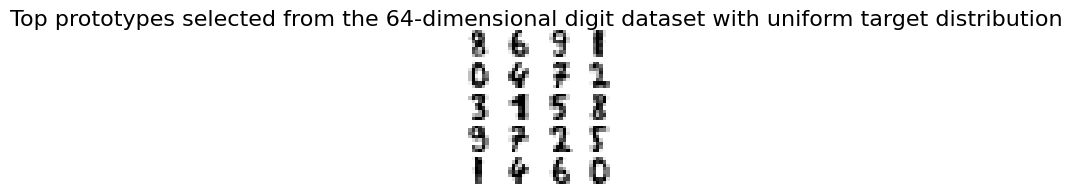
targetmarginal 是目标点上的经验分布。通常假定它是均匀分布的，即每个目标点具有同等重要性。在实验中，我们讨论了两种设置。第一种设置中，我们将 targetmarginal 设为均匀分布。第二种设置中，我们将 targetmarginal 偏向特定类别的点。实验表明，在这两种设置下，学习到的原型都能很好地代表目标分布 targetmarginal。

设置 1：目标分布是均匀的

# Define a targetmarginal on the target set
# We define the uniform marginal
targetmarginal = np.ones(C.shape[1])/C.shape[1];


# The number of prototypes to be computed
numprototypes = 20;

# Run SPOTgreedy
# prototypeIndices represent the indices corresponding to the chosen prototypes.
# prototypeWeights represent the weights associated with each of the chosen prototypes. The weights sum to 1. 
[prototypeIndices, prototypeWeights] = SPOT_GreedySubsetSelection(C, targetmarginal, numprototypes);

# Plot the chosen prototypes
fig, axs = plt.subplots(nrows=5, ncols=4, figsize=(2, 2))
for idx, ax in enumerate(axs.ravel()):
    ax.imshow(data[prototypeIndices[idx]].reshape((8, 8)), cmap=plt.cm.binary)
    ax.axis("off")
_ = fig.suptitle("Top prototypes selected from the 64-dimensional digit dataset with uniform target distribution", fontsize=16)

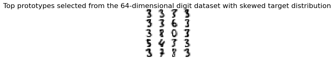
设置 2：目标分布是偏斜的

在此设置中，我们将 tgt 中对应标签 3 的示例偏斜了 90%。我们期望学习到的原型中有很大一部分也属于标签 3。

# Skew the target marginal to give weights to specific classes more
result = np.where(y_tgt == 3); # find indices corresponding to label 3.


targetmarginal_skewed = np.ones(C.shape[1]);
targetmarginal_skewed[result[0]] = 90; # Weigh the instances corresponding to label 3 more.
targetmarginal_skewed = targetmarginal_skewed/np.sum(targetmarginal_skewed);

# Run SPOTgreedy
[prototypeIndices_skewed, prototypeWeights_skewed] = SPOT_GreedySubsetSelection(C, targetmarginal_skewed, numprototypes);

# Plot the prototypes selected
fig, axs = plt.subplots(nrows=5, ncols=4, figsize=(2, 2))
for idx, ax in enumerate(axs.ravel()):
    ax.imshow(data[prototypeIndices_skewed[idx]].reshape((8, 8)), cmap=plt.cm.binary)
    ax.axis("off")
_ = fig.suptitle("Top prototypes selected from the 64-dimensional digit dataset with skewed target distribution", fontsize=16)